
Let a small number of connections carry a high-rank update.
Consider a weight matrix with 4,096 inputs and 4,096 outputs. Suppose we want to change every diagonal entry and leave every other entry untouched:
This update changes 4,096 connections. Its rank is also 4,096.
A coordinate representation expresses it with 4,096 trainable values. A standard LoRA parameterization with rank 16 uses 131,072 factor values and leaves 99.6% of the target’s squared Frobenius norm unexplained. To represent the target exactly, the two LoRA factors require rank 4,096 and contain 33,554,432 values.
The difference comes from the structure of the update. A small number of independent connection changes can form a full-rank matrix.
Parameter efficiency and low rank are different properties.
SparseLeaf starts from this distinction. It freezes a pretrained network, gives a selected set of existing connections independent trainable increments, and optimizes those increments directly. The entire network supplies its computation; a small set of connections supplies its plasticity.
We call this synaptic sparse fine-tuning. Its central principle is simple:
Constrain how many connections can change. Preserve the freedom for those changes to form a high-rank update.
1. Why LoRA Is Wrong: Parameter Efficiency Is Not Low Rank
Two different constraints
Write the adapted weight matrix as
where \(W_0\) is the pretrained weight and \(\Delta W\) is the accumulated change introduced by learning.
There are two distinct ways to constrain this change:
The first limits the number of independent matrix directions. The second limits the number of weight coordinates that change.
A dense outer product \(uv^\top\) can modify every entry while having rank one. A diagonal matrix with nonzero diagonal entries changes very few entries while having full rank. Sparsity describes where changes occur; rank describes how many independent directions they contain.
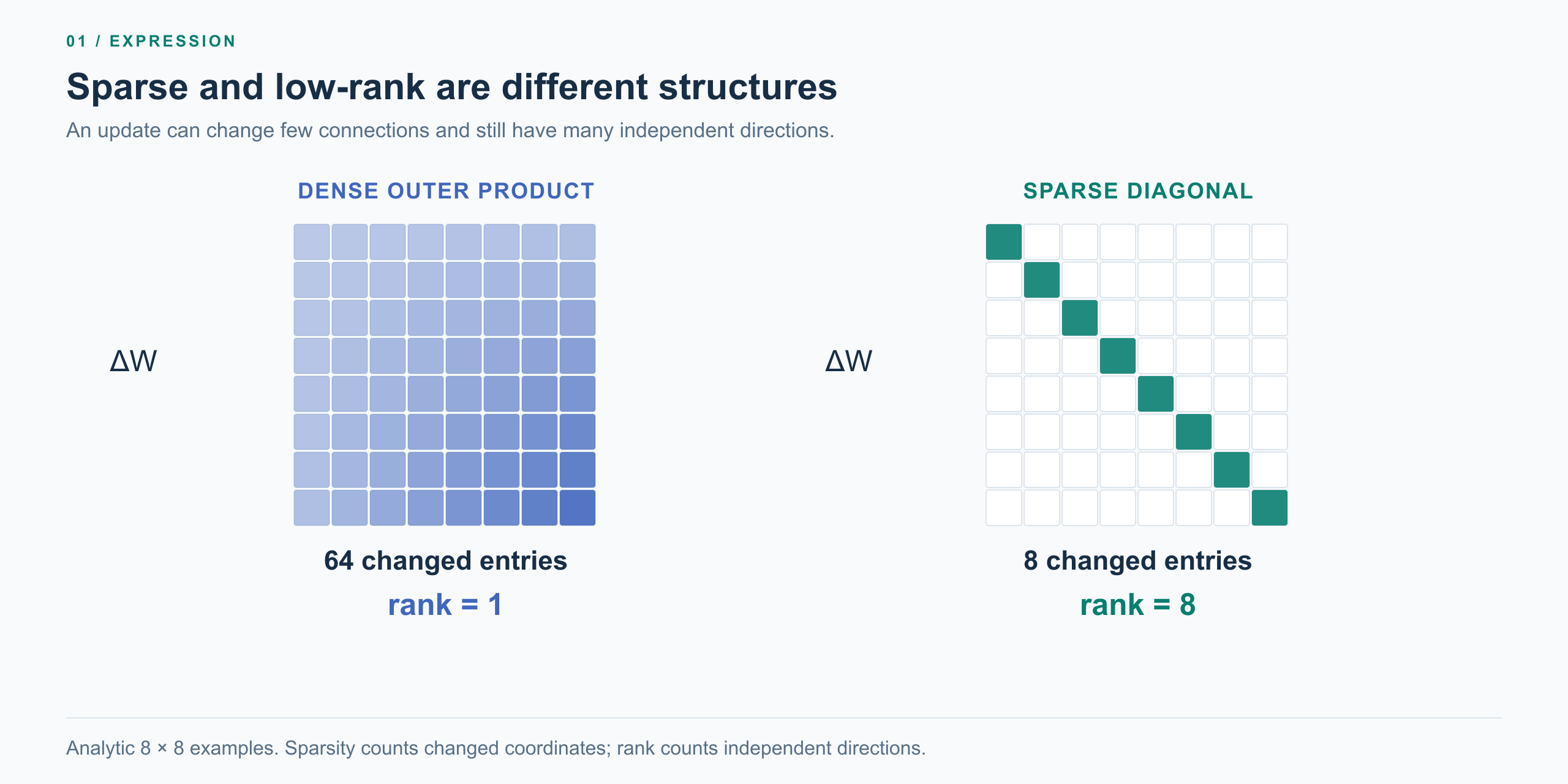
Figure 1. Two different structures. The outer product changes all 64 entries and has rank one. The diagonal update changes eight entries and has rank eight. These are analytic examples of update matrices.
The expressive price of factorization
LoRA represents the update to an \(m\times n\) weight matrix through two trainable factors:
It stores \(r(m+n)\) trainable factor values and enforces \(\operatorname{rank}(\Delta W)\le r\). This is the low-rank parameterization introduced by Hu and colleagues in LoRA.
For an input \(x\), the output correction is
Every correction passes through an \(r\)-dimensional intermediate representation and lies in the column space of \(B\). Training can rotate that space; its dimension remains at most \(r\).
The factors also couple the changes made to individual connections. Changing one entry of \(B\) changes a row pattern determined by \(A\). Changing one entry of \(A\) changes a column pattern determined by \(B\). Learning operates through shared patterns of connection changes.
Now consider the family
Each of its \(d\) connections has an independent adjustment. The family has \(d\) scalar degrees of freedom, and every member has rank \(d\).
Coordinate learning assigns one variable to each adjustment. Standard LoRA needs \(r\ge d\) to express these matrices exactly, at which point its two factors contain at least \(2d^2\) values.
This is the central criticism: a low-rank parameterization turns a restriction on learning variables into a restriction on independent update directions. For sparse, independent corrections, rank is the wrong quantity to ration.
The expressive loss has an exact form. By the Eckart–Young low-rank approximation theorem, if the target update has singular values \(\sigma_1\ge\sigma_2\ge\cdots\), its best rank-\(r\) approximation satisfies
The discarded singular directions have a price even at the best possible solution. Zeng and Lee make this relationship explicit in their analysis of LoRA’s expressive power: their deep-linear theorem characterizes the optimal approximation error through the singular spectrum of the target correction and identifies the adapter rank needed for exact representation. Rank is an expressivity budget. The Expressive Power of Low-Rank Adaptation, §2
For \(\Delta W^*=aI_d\), all \(d\) singular values equal \(|a|\). The fraction of squared update energy left out is
Low intrinsic dimension is not low matrix rank
The literature on intrinsic dimension asks how many trainable variables are needed to adapt a pretrained model. Aghajanyan, Gupta, and Zettlemoyer report that 200 variables, mapped into the full parameter space through a random projection, achieve 90% of full-parameter fine-tuning performance on MRPC with RoBERTa. Their experiments also show that pretraining reduces the measured intrinsic dimension of adaptation. Intrinsic Dimensionality Explains the Effectiveness of Language Model Fine-Tuning
This is a statement about the dimension of the learning parameterization. Matrix rank measures something else: the number of independent directions in a particular layer’s update. Our diagonal family makes the separation explicit—\(d\) learning variables produce rank-\(d\) matrices. A compact adaptation can carry a high-rank transformation.
Independent connection adjustments do not become redundant merely because we want a small training state. SparseLeaf keeps those adjustments independent and places the budget on their count.
Zero output can hide an inactive learning path
Factorization imposes a second cost before learning has made its first update. The standard initialization sets \(B_0=0\) and draws \(A_0\) randomly, making \(B_0A_0=0\). This is the zero-product initialization specified in the original LoRA paper. Hu et al., §4.1 It preserves the pretrained model’s initial function. It does not preserve its learning geometry.
Take unit adapter scaling and write \(G=\nabla_W\mathcal L\). The factor gradients are
At initialization,
The entire \(A\) block receives no task gradient on the first backward pass. Learning initially changes how the random features are combined through \(B\); changing the features through \(A\) depends on \(B\) first becoming nonzero.
Setting both factors to zero makes both gradients zero. Gradient descent and Adam with zero initial moments then remain at that point. A zero product and a trainable zero increment are fundamentally different constructions.
The differential makes the inactive path explicit:
For a full-row-rank \(A_0\), the initial parameter-to-weight Jacobian has rank \(mr\). LoRA stores \(r(m+n)\) factor values, but all \(rn\) coordinates of \(A\) are invisible to this initial differential. The parameter count overstates the number of independent directions available at the starting point.
The random basis decides what can move first
The initial tangent space—the weight changes available to first order—is
Every row of an initial correction lies in the row space of \(A_0\). For an input direction \(v\) with \(A_0v=0\), every correction in \(\mathcal T_0\) satisfies \((HA_0)v=0\). At rank \(r<n\), there are at least \(n-r\) such independent input directions.
This is an initialization bottleneck as well as a rank bottleneck: the first corrections must pass through a randomly chosen set of input directions. The task cannot immediately use arbitrary directions within the eventual rank-\(r\) model family. Learning the basis itself starts through the other factor’s learning.
Even exchanging the zero and random factors changes the dynamics. Hayou, Ghosh, and Yu derive different stable learning-rate scalings and observe different fine-tuning performance for these two initializations, despite identical initial model outputs. Starting from the same function does not mean starting with the same ability to learn. The Impact of Initialization on LoRA Finetuning Dynamics
Zero the increment, not its derivative
SparseLeaf gives each selected connection its own increment:
Its derivative is already present at zero:
All selected connection directions are available from the first backward pass. Zero increments preserve the pretrained function without silencing a parameter block or introducing a random learned basis between the task gradient and its trainable variables.
The support determines where learning is allowed. The native gradient determines how each permitted connection should change. SparseLeaf starts with both parts of that interface intact.
2. SparseLeaf: Give Existing Connections Plasticity
In a neural layer,
the scalar \(W_{ij}\) is the connection from input activation \(x_j\) to output unit \(i\). Selecting that coordinate for training gives that connection the ability to change its strength.
The synaptic perspective has a concrete biological motivation. In hippocampal neurons, Matsuzaki and colleagues induced potentiation at individual dendritic spines: structural enlargement and increased AMPA-receptor currents were localized to the stimulated spine, with neighboring spines unaffected. The individual connection can be a unit of plasticity. SparseLeaf takes that connection-level viewpoint as its organizing principle for fine-tuning. Structural basis of long-term potentiation in single dendritic spines
For a frozen matrix \(W_0\in\mathbb R^{m\times n}\), choose \(K\) distinct coordinates:
Associate an independent increment \(\theta_k\) with each selected connection:
The trainable vector is \(\theta\in\mathbb R^K\). We initialize it at zero, so learning starts from the pretrained model.
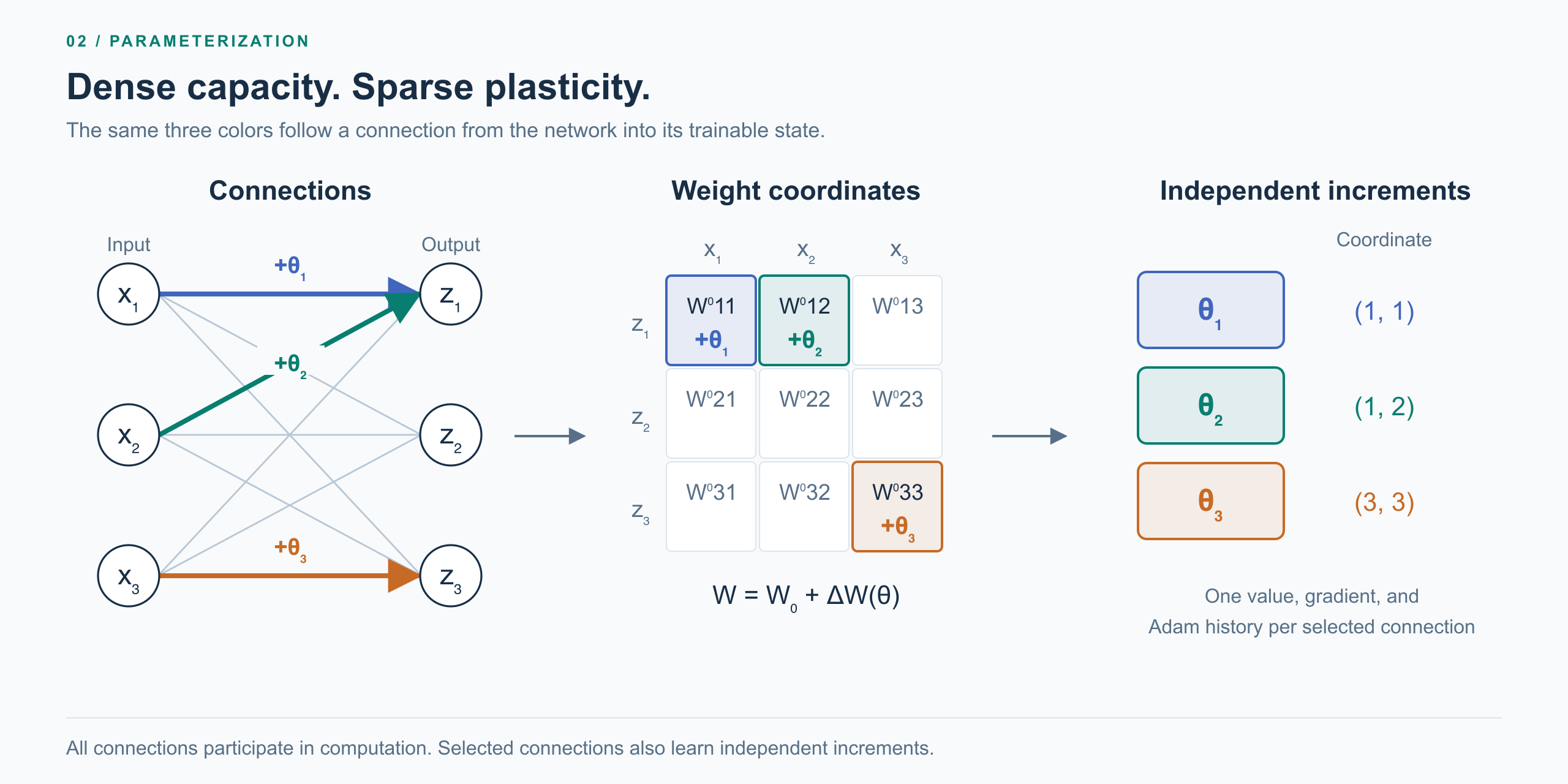
Figure 2. One set of connections, three views. Gray connections retain their pretrained weights and participate in computation. Colored connections use their pretrained weights plus independent increments. The same colors identify the connections, matrix entries, and trainable values.
This separates two roles that are often bundled together. The dense network provides the representational machinery built during pretraining. The selected connections provide the degrees of freedom used to adapt that machinery.
Dense capacity. Sparse plasticity.
Sparsity as an optimization constraint
The underlying optimization problem is
There are two decisions inside this problem: where plasticity is allocated, and what values the plastic connections learn. SparseLeaf makes these decisions explicit. It chooses a support \(S\), then solves
For a fixed support, this is learning in a coordinate subspace. Each trainable direction is an original weight coordinate, and each variable controls exactly one connection.
The largest rank attainable by an \(m\times n\) matrix with at most \(K\) nonzero entries is
Placing nonzero entries on distinct rows and columns attains this maximum. In a square layer, a diagonal support reaches full rank with only one trainable connection per row and column.
The support remains fixed during training, so both the accumulated change \(W_t-W_0\) and every step \(W_{t+1}-W_t\) stay within the same set of \(K\) connections. The sparsity budget organizes the entire learning trajectory.
Sparse changes are a learning primitive
Diff Pruning formulates adaptation as a sparse additive difference from frozen pretrained parameters, using a differentiable approximation to an \(L_0\) penalty to learn the support. Its structured variant modifies 0.5% of BERT-Large’s parameters and matches its full-fine-tuning baseline’s reported GLUE average of 80.6, excluding QNLI from that average. The full network remains available while the task-specific change is sparse. Guo, Rush, and Kim, Table 1
SpaRTA takes an even simpler route: randomly select a small set of original parameters and train their increments while freezing the rest. Its Gemma and Mistral experiments find competitive performance with LoRA at similar trainable-parameter counts. This provides a direct empirical example of parameter-efficient adaptation built from coordinate sparsity. Rios et al., Sparsity May Be All You Need
These methods establish the usefulness of sparse changes. SparseLeaf organizes that idea around independent plastic connections, a fixed support, and an optimizer whose entire trainable state lives on that support.
3. When High-Rank Sparse Learning Beats Low-Rank Dense Learning
We can turn the expressive difference into an exact learning result.
Consider a \(d\times d\) linear layer. Draw inputs with second moment
and define the target by
Every input coordinate requires its own adjustment. With squared loss,
SparseLeaf follows the full-gradient trajectory
Select the \(d\) diagonal coordinates and initialize all increments at zero. Use the exact gradient of this population loss, ordinary gradient descent, and a constant step size \(0<\eta<2\).
Each selected increment follows
Therefore,
and
The full gradient is diagonal throughout this trajectory. SparseLeaf learns every coordinate that the full update changes, producing the same weights at every step.
Low rank leaves a positive minimum loss
A LoRA update satisfies \(\operatorname{rank}(BA)\le r\). For \(r<d\), the best achievable loss is
This is the global minimum over the factors. Optimization within the rank-\(r\) family cannot remove the error associated with the remaining \(d-r\) directions.
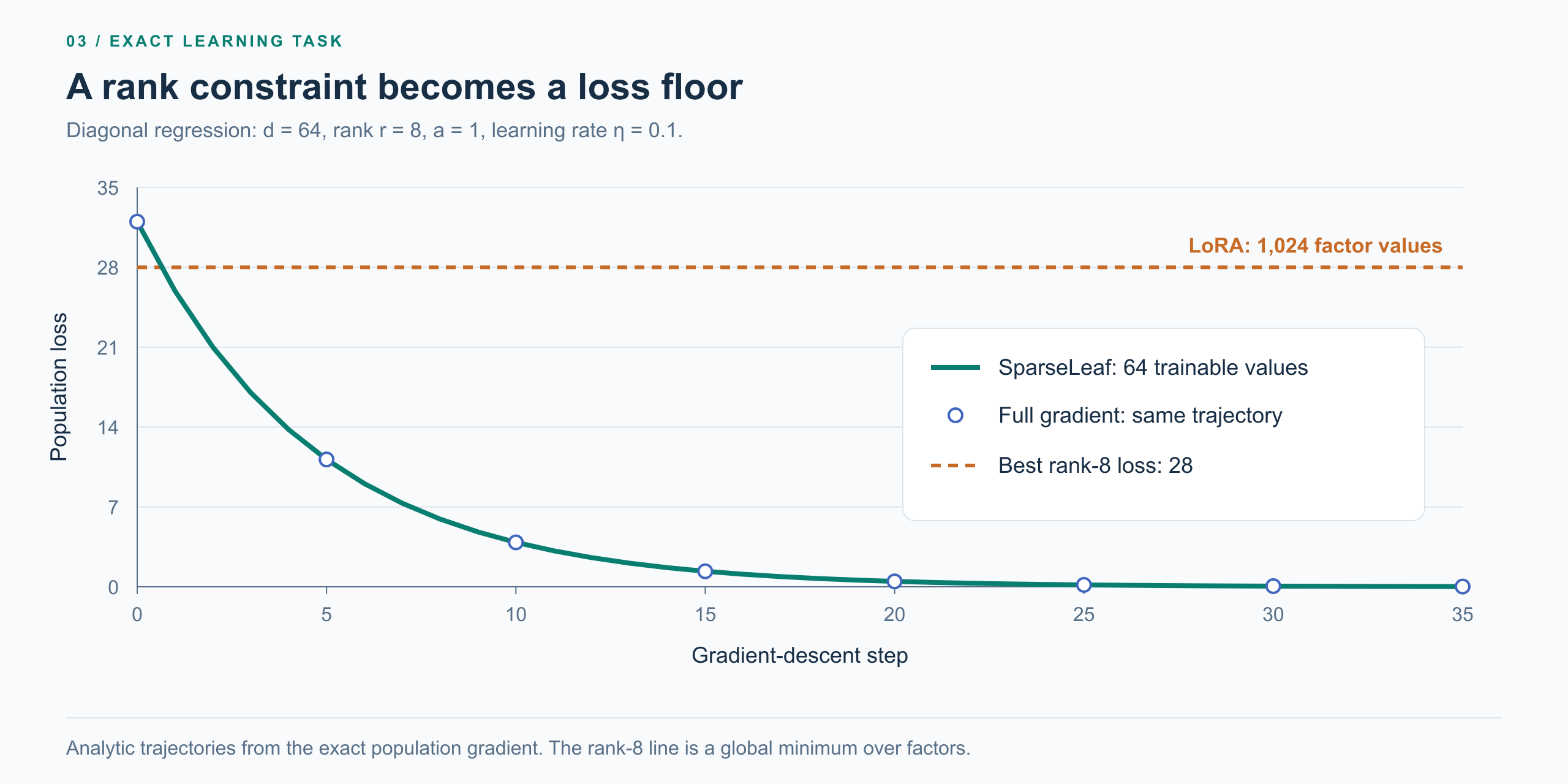
Figure 3. Analytic regression example with \(d=64\), \(r=8\), \(a=1\), and \(\eta=0.1\). SparseLeaf and full-gradient descent have the same trajectory. The orange line is the best loss achievable by any rank-eight update.
The comparison is unusually direct. SparseLeaf learns \(d\) values and reaches zero loss. Standard LoRA learns \(2dr\) factor values and retains a positive loss floor.
The target is simple in coordinates and rich in independent directions. A sparse parameterization captures both facts at once.
High-rank sparse learning wins here because it allocates variables to the changes the task actually requires.
The empirical counterpart
Sparse high-rank adaptation also wins direct comparisons in language models. In Bhardwaj and colleagues’ SHiRA experiments, LLaMA-7B reaches 77.4% average accuracy across eight commonsense-reasoning benchmarks with SHiRA-SNIP, compared with 74.7% for LoRA. SHiRA trains 1.0% of the original parameters; LoRA uses 0.83% in trainable factors. The magnitude-selected SHiRA variant reaches 77.0%. Sparse High Rank Adapters, Table 2
Liu and colleagues report a matched-parameter comparison on Gemma2-2B, trained on MetaMathQA and evaluated on five-shot GSM8K. Their static, gradient-selected sparse adaptation scores 50.27% versus LoRA’s 39.20% with flexible answer extraction, and 37.15% versus 28.81% with strict matching. The trainable budget is held equal while its parameterization changes. Refining Salience-Aware Sparse Fine-Tuning Strategies for Language Models, Table 3
The analytic task explains an expressive advantage of sparse, independent corrections. These published comparisons show that coordinate-sparse adaptation can turn its learning budget into better task performance than low-rank factorization.
4. SparseLeaf Adam: Optimize the Connections Directly
Expressive capacity determines which changes are available. Parameterization also determines how learning signals reach those changes.
Flatten the weights into \(w\in\mathbb R^N\). Let \(P_S\in\mathbb R^{K\times N}\) extract the selected coordinates. SparseLeaf writes
The chain rule gives
Each increment receives the gradient of its own weight coordinate, evaluated at the current adapted model.
The optimizer
Initialize \(\theta_0=m_0=v_0=0\). At training step \(t\ge1\), compute
Maintain the first and second moments in the selected coordinate space:
Apply bias correction,
and update
Products, powers, square roots, and division in the optimizer are elementwise. These are Adam’s moment updates, applied directly to the \(K\) plastic connections.
There is a useful optimization interpretation. Define
Then the increment \(u_t=\theta_t-\theta_{t-1}\) solves
The support specifies which connections may move. The adaptive metric specifies the scale of movement along each permitted direction. Sparsity is built into the feasible space of the optimizer.
This quadratic-step viewpoint connects SparseLeaf Adam to adaptive proximal optimization. Duchi, Hazan, and Singer developed methods in which gradient history changes the geometry used to measure a step. Here, that adaptive geometry is defined directly on the selected connections: the support chooses the axes, and each connection’s second-moment history sets its metric weight. Adaptive Subgradient Methods for Online Learning and Stochastic Optimization
Native coordinates preserve native geometry
Because the selected coordinates are distinct,
The embedding preserves lengths and inner products. A scalar increment has the same meaning in the learning vector and in the weight matrix.
For a clean comparison, consider one ordinary gradient-descent step at the same current weights, with gradient \(g\). Full-parameter gradient descent takes \(-\eta g\); SparseLeaf takes \(-\eta P_S^\top P_Sg\). Their squared difference is exactly
Every selected coordinate receives its original gradient. The discrepancy is the gradient energy outside the selected support. When the full-gradient trajectory stays within \(S\), identical initialization and training steps give identical trajectories by induction. The diagonal task above makes this identity explicit.
Initialization determines the first learning geometry
We can now quantify the initialization bottleneck from Section 1. Take unit adapter scaling, no adapter dropout, and ordinary gradient descent. At the base model, let \(G=\nabla_W\mathcal L(W_0)\), draw \(A_0\) randomly, and set \(B_0=0\). Since the first task gradient of \(A\) is zero, \(A_1=A_0\), while \(B_1=-\eta GA_0^\top\). The first effective weight update is exactly
The gradient passes through the random Gram matrix \(A_0^\top A_0\). Its scale and directional weighting come from the initialization. Replacing \(A_0\) with \(cA_0\) leaves the initial model unchanged but multiplies this SGD update by \(c^2\) at the same learning rate. Initialization therefore changes the effective optimizer while keeping the starting predictions identical.
Flora develops this connection into a random-projection interpretation of LoRA’s SGD dynamics. It then refreshes the projections to obtain high-rank accumulated updates while keeping optimizer states compact. The distinction is fundamental: compressing the state used to learn and restricting the rank of the accumulated change are different design decisions. Flora, §§2–3
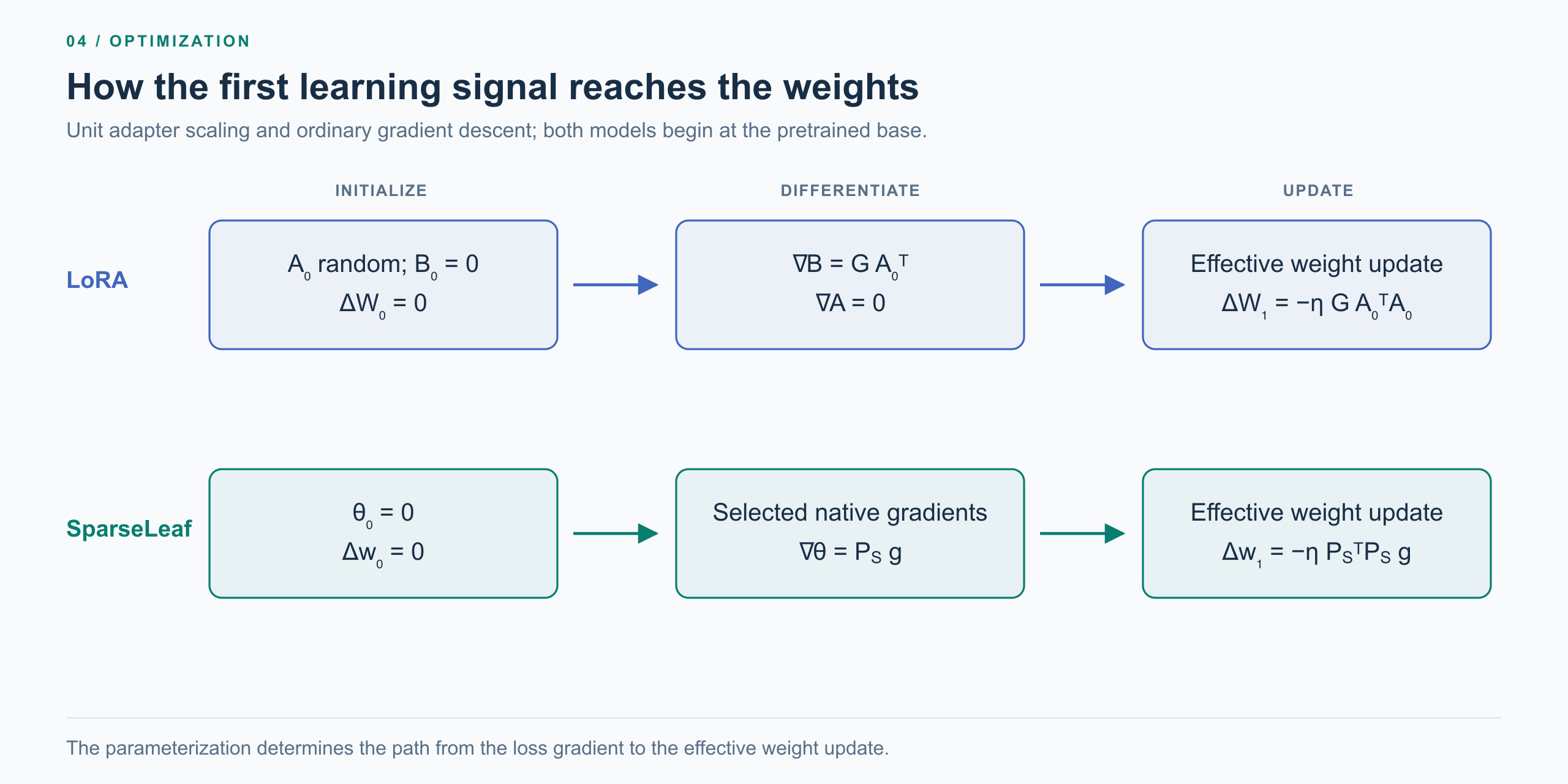
Figure 4. Both parameterizations start at the base model. With unit adapter scaling and ordinary gradient descent, LoRA’s first effective update is \(-\eta GA_0^\top A_0\); SparseLeaf’s is \(-\eta P_S^\top P_Sg\) in flattened coordinates.
To isolate random geometry from mean scale, use independent \(A_{0,ij}\sim\mathcal N(0,1/r)\) and fixed \(G\). This normalization gives \(\mathbb E[A_0^\top A_0]=I_n\), so the mean first update is \(-\eta G\). Its mean squared deviation from that update is
For \(n=4096\) and \(r=8\), the relative mean squared deviation is \(4097/8=512.125\). Matching the full-gradient step in expectation says little about the step produced by one initialized adapter. Appendix A gives the exact calculation.
The adapter’s external multiplier introduces another scale coupling. Write the adapter as \(\gamma_r BA\), keep \(B_0=0\), and now use independent, zero-mean entries of \(A_0\) with variance \(\sigma_A^2\) independent of \(r\). The same first-step SGD calculation gives
With fixed \(\alpha\), the usual \(\gamma_r=\alpha/r\) makes this mean step shrink as \(1/r\); \(\gamma_r=\alpha/\sqrt r\) keeps its scale constant. The rsLoRA paper derives the square-root rule through a rank-stability analysis and demonstrates improved use of larger ranks. Rank is entangled with optimization scale before its additional capacity can be used. A Rank Stabilization Scaling Factor for Fine-Tuning with LoRA, §3 and Appendix A
Better scaling cannot restore missing directions
Remove the random singular-value scaling and examine the initial subspace itself. For full-row-rank \(A_0\), its orthogonal projector is
The closest approximation to \(G\) inside \(\mathcal T_0\) is \(G\Pi_0\). An isotropic Gaussian initialization chooses a uniformly oriented \(r\)-dimensional row space, giving
At width 4096 and rank 8, the initial tangent space captures 0.1953% of a fixed task gradient’s squared energy on average. This is the best projection into that initial space, with its conditioning already removed. Rescaling a step cannot recover the missing directions; they require learning a different basis.
The two factors also control that basis learning through one another. With SGD learning rates \(\eta_A,\eta_B\) and \(G_t=\nabla_W\mathcal L(W_t)\), the second update gives
Its onset is coupled to both learning rates. LoRA+ analyzes this imbalance in the large-width limit and uses different factor learning rates to improve feature learning. The factors require a relative learning-rate choice in addition to the choice of starting basis. LoRA+: Efficient Low Rank Adaptation of Large Models
Adam normalizes factor gradients inside the same initial subspace
The first-step geometry remains explicit with Adam. Start both factors’ optimizer moments at zero and define \(\Gamma_0=GA_0^\top\). Bias correction gives \(\widehat m_{B,1}=\Gamma_0\) and \(\widehat v_{B,1}=\Gamma_0^{\odot2}\). The resulting unit-scaled adapter is
Adam changes the coefficients multiplying \(A_0\). Every row of this first update still belongs to its initial row space, and \(A\) still receives zero task gradient at the starting point. Factorwise normalization does not create directions absent from that space.
There is a second problem with factorwise normalization. The same product has equivalent representations \(BA=(BR)(R^{-1}A)\) for any invertible \(R\). Yen and colleagues show that gradient descent and Adam generally produce different effective weight updates from equivalent factorizations. Their LoRA-RITE optimizer introduces matrix preconditioning to restore transformation invariance. Normalizing factor gradients is not the same as normalizing changes to the model. LoRA Done RITE, §§2–3
For SparseLeaf, let \(g_S=P_Sg\) at the same pretrained model. Its first Adam update is
Every selected connection is normalized using its own task gradient. The embedding has \(K\) orthonormal coordinate directions even at \(\theta=0\). There is no factor whose zero value blocks another factor’s learning, and no random Gram matrix to insert between the selected gradient and its update. For a fixed support and coordinate ordering, each sparse increment has one parameter vector; there is no equivalent-factor scaling or rotation for the optimizer to reconcile.
Initialization research identifies the cost of the extra basis
LoRA-Pro states the optimization problem directly in weight space. It adjusts factor gradients to minimize the difference between their induced weight differential and the full-fine-tuning gradient. The factorized parameterization introduces a gradient-approximation problem inside the learning procedure itself. LoRA-Pro, §§2.2–2.3
LoRA-GA explicitly targets the mismatch between LoRA’s initial weight-update direction and the full-fine-tuning gradient. It initializes the factors from singular vectors of a sampled task gradient and offsets the frozen weight to preserve the initial model. LoRA-GA, §§3.2–3.4
PiSSA instead initializes the factors from principal components of the pretrained weight and freezes its residual. The initial function is preserved, but the basis now comes from the pretrained matrix rather than a random draw. PiSSA, §3
EVA uses a third source of directions: the pretrained model’s input activations on task data. It initializes \(A\) from their leading right singular vectors and keeps \(B_0=0\). Its \(\rho=1\) configuration retains uniform ranks, giving a direct comparison of activation-based and random initialization at the same parameter count. Explained Variance Adaptation, §§3.2–3.5
Published experiments make the consequences concrete. Each row below is a comparison within the cited study; the reported results are task accuracies.
| Factorization choice tested | Model and training setup | Reported result |
|---|---|---|
| Which factor starts at zero | RoBERTa-large on MNLI; \(r=8\), FP16, three seeds; learning rate searched for each initialization | \(A_0=0\): 89.47%; \(B_0=0\): 90.69%. Hayou et al., §4.1 and Figure 4 |
| Gradient-aligned initialization and stable scaling | Llama-2-7B, MetaMathQA training, GSM8K evaluation; \(r=8\), three seeds | LoRA: 42.08% → LoRA-GA: 53.60%. LoRA-GA, Table 2 |
| Activation-based initialization at fixed rank and parameter count | Llama-2-7B, MetaMathQA training, GSM8K evaluation; \(r=16\), 40.6M trainable parameters each, three seeds | LoRA: 59.7% → EVA (\(\rho=1\)): 61.9%. EVA, Table 11 |
| Transformation-invariant factor optimization | Gemma-7B on GSM8K; \(r=16\); learning rate searched for each optimizer | Adam: 48.37% → LoRA-RITE: 55.50%. LoRA-RITE, §5 and Table 2 |
Together with LoRA+, these studies identify the optimization work introduced by factorization: choose a basis, calibrate its scale, balance its factors, and correct the geometry of their updates. SparseLeaf places the design decision directly on the support. Once the connections are selected, zero increments and zero Adam moments are enough to start learning in their native coordinates. Preserve the pretrained computation, and spend the learning budget on independently changing its connections.
The difference is visible in learned weights as well. Shuttleworth and colleagues find that LoRA and full fine-tuning produce distinct spectral structures even at similar downstream performance. LoRA introduces prominent singular vectors that differ sharply from those of the pretrained model, which the authors call intruder dimensions. A parameterization shapes both the path of learning and the structure of its solution. LoRA vs Full Fine-tuning: An Illusion of Equivalence, §3
Backpropagation at connection granularity
For a token batch \(X\in\mathbb R^{T\times n}\) and upstream gradient \(D\in\mathbb R^{T\times m}\), the selected parameter gradient is
The implementation can compute these \(K\) inner products directly. Error signals continue through the full effective layer:
The resulting learning rule is local in its parameterization and network-wide in its computation. Each plastic connection has its own value, gradient, and adaptive history; the surrounding network continues to participate in the forward and backward passes.
5. Which Connections Should Be Plastic?
Once sparsity becomes an optimization constraint, support selection becomes a question about learning: which connections can jointly produce the changes a task requires?
Pretrained computation provides the substrate
A pretrained model already contains a large, organized system of features and transformations. Fine-tuning changes how that system responds to a task. An adjustment to an early connection can influence many downstream activations; adjustments across different layers can work together through the existing computation.
The learning signal on a connection has a precise form. For one input, write \(\delta_i=\partial\mathcal L/\partial z_i\). Then
Across the task distribution, the persistent signal is
Input activity and output error jointly determine which connections receive consistent pressure to change. Adam’s first moment accumulates direction over time, while its second moment tracks gradient magnitude. The learning history of each selected connection becomes part of its adaptive update rule.
Reward selects useful changes
For on-policy learning with a parameter-independent reward, let
The REINFORCE score-function estimator connects expected reward to connection-level updates. The score-function identity gives \(\mathbb E[s_i\mid x]=0\). With the conditional mean reward as a baseline, the expected policy gradient can be written as
A connection receives a sustained reward-learning signal when its influence on action probabilities correlates with reward. Positive and negative contributions can cancel on other connections. This connects plasticity to the task’s preferred changes in behavior.
Sparse, high-rank updates are also visible in empirical analyses of RL-trained language models. Mukherjee and colleagues examined ten models and seven RL algorithms. In their BF16 checkpoint analysis, using a \(10^{-5}\) change tolerance, 68.5%–96.0% of parameters remained unchanged after RL. The four model–algorithm combinations in their rank table had mean update ranks of 99.2%–99.8% of the maximum. They also retrained identified subnetworks in DPO and PRIME experiments and recovered or improved the reported task scores. These observations put sparse plasticity and high-rank updates in the same empirical picture. Reinforcement Learning Finetunes Small Subnetworks in Large Language Models, §§3–4
A support must cover the task’s required changes
Stack the model’s outputs over the task data and linearize around the pretrained parameters:
A selected support gives the output change \(J_S\theta\). For a desired local output correction \(b\), consider
The optimal residual is
This makes the role of support selection concrete. The selected connections should jointly span the changes that matter to the task.
There is also a function-space interpretation. The neural tangent kernel expresses how parameter gradients combine to move a model’s outputs. Jacot, Gabriel, and Hongler, §4 In the local model above, the kernel available to SparseLeaf is
For gradient flow on \(\tfrac12\|J_S\theta-b\|_2^2\), the residual \(e=J_S\theta-b\) follows
Selecting plastic connections selects the Jacobian features that build this learning kernel. Their joint span determines which output errors can be removed; their kernel eigenvalues determine how quickly those errors decay in the local model. Support selection therefore shapes both the available changes and the dynamics of learning them.
Take four candidate coordinates with output effects
With a budget of two coordinates, selecting the first two gives two controls along the same output direction and leaves residual \((0,1)^\top\). Selecting the first and third covers the target exactly.
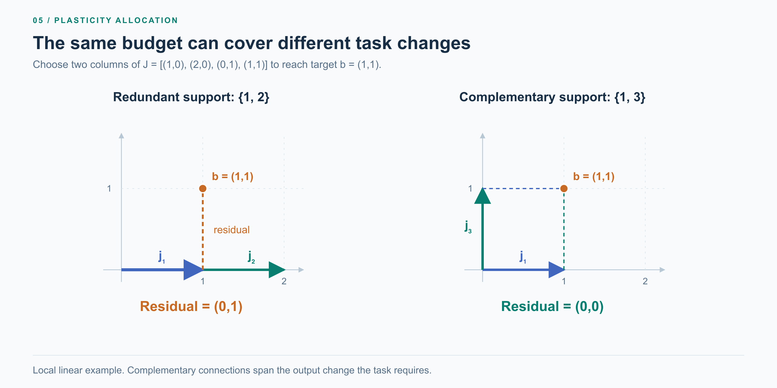
Figure 5. Support quality depends on the combined effect of its connections. Both choices use two trainable values; the complementary support covers the two-dimensional target.
The value of a connection depends on the changes it enables together with the other plastic connections.
Allocate plasticity by its learning value
A local quadratic model makes support selection an explicit optimization problem:
For a support \(S\) with positive-definite \(H_{SS}\), the optimal supported step and its predicted improvement are
The allocation problem is therefore
With positive diagonal curvature, each coordinate receives score \(g_i^2/(2h_i)\). For example:
| Coordinate | Gradient \(g_i\) | Curvature \(h_i\) | Optimal quadratic improvement |
|---|---|---|---|
| 1 | −4 | 16 | 0.5 |
| 2 | −3 | 3 | 1.5 |
| 3 | −2 | 1 | 2.0 |
| 4 | −1 | 0.1 | 5.0 |
With one plastic connection, the largest gradient selects coordinate 1. The greatest predicted improvement selects coordinate 4. Curvature and task coverage give structure to the question of where learning should happen.
Coordinate-optimization theory gives this principle a concrete rule. Nutini and colleagues’ Gauss–Southwell–Lipschitz rule selects the coordinate maximizing \(|g_i|/\sqrt{L_i}\), where \(L_i\) measures coordinate-wise smoothness. For the diagonal quadratic above, \(L_i=h_i\), so it selects exactly the coordinate with the greatest \(g_i^2/(2h_i)\) improvement. Coordinate Descent Converges Faster with the Gauss-Southwell Rule Than Random Selection, §6.2
For neural-network adaptation, FISH Mask estimates diagonal Fisher information, selects the \(K\) largest entries, and reuses that fixed mask during training. It makes task sensitivity an explicit criterion for assigning plasticity. Sung, Nair, and Raffel, Training Neural Networks with Fixed Sparse Masks Liu and colleagues subsequently compare eight salience metrics and static versus dynamic masking; their results identify a simple gradient-based static mask as a strong sparse-adaptation strategy. Refining Salience-Aware Sparse Fine-Tuning Strategies, §§3–4
The experiments below use a concrete, reproducible allocation rule: within each target matrix’s budget, select the largest-magnitude pretrained weights and keep that support fixed. A chunked Top-K procedure determines the coordinates; training then updates their increments and moment states.
Selection determines where learning may occur. The gradients determine how those connections change.
6. What a Small Set of Connections Learns
The experiments express learning capacity through a direct variable: the number of plastic connections.
Supervised fine-tuning: the plasticity–quality curve
On Qwen3-1.7B, the GSM8K experiment uses completion-only supervised fine-tuning for 2,048 steps, batch size 2, and maximum sequence length 256. Validation measures completion-only negative log-likelihood on a held-out slice. Density is the proportion of coordinates selected within the targeted linear matrices.
| Trainable coordinates \(K\) | Density | Seeds | Validation NLL ↓ |
|---|---|---|---|
| 1,525,311 | 0.10823% | 3 | 0.4158 ± 0.0013 |
| 653,576 | 0.04638% | 5 | 0.4164 ± 0.0010 |
| 352,212 | 0.02499% | 2 | 0.4215 ± 0.0010 |
| 217,812 | 0.01546% | 3 | 0.4284 ± 0.0010 |
| 70,364 | 0.00499% | 3 | 0.4499 ± 0.0015 |
| 28,028 | 0.00199% | 3 | 0.4752 ± 0.0010 |
The ± values are sample standard deviations across seeds. The base model’s NLL is 1.5935. The reported LoRA \(r=8\) reference has mean NLL 0.4329 across three seeds.
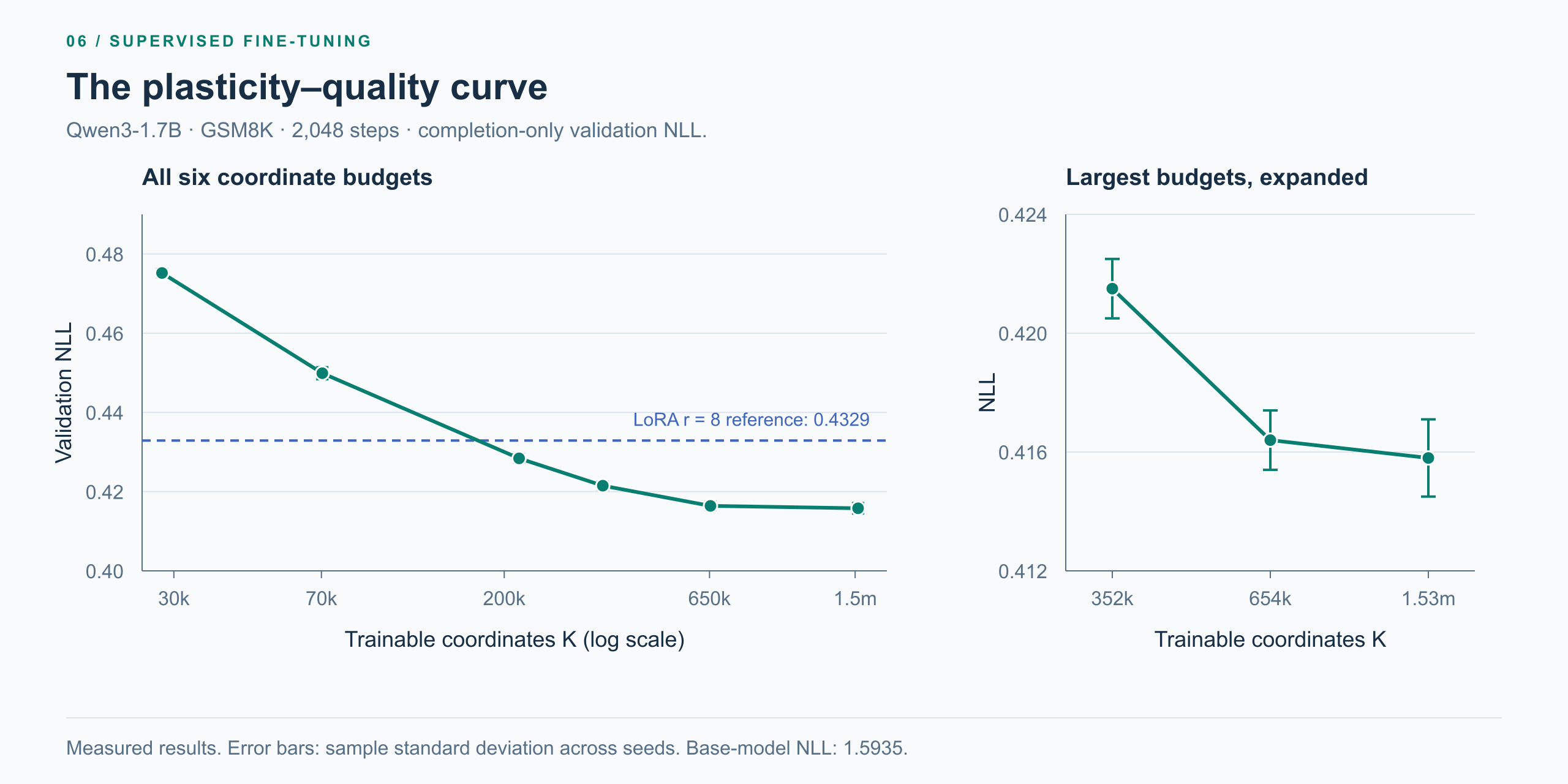
Figure 6. The plasticity–quality curve. The left panel shows all six coordinate budgets on a logarithmic horizontal axis; the right panel expands the three largest budgets. Error bars are sample standard deviations. The horizontal reference marks LoRA \(r=8\) at NLL 0.4329.
Three features of this curve explain the role of the learning budget.
First, 28,028 plastic connections produce a substantial change in task fit: NLL falls from 1.5935 to 0.4752. A pretrained model can be adapted through a very small set of connection adjustments.
Second, increasing the support expands the available adaptation. Moving from 28,028 to 352,212 coordinates lowers NLL from 0.4752 to 0.4215.
Third, the curve flattens. Reducing the budget from 1,525,311 to 653,576 removes approximately 57% of the trainable values, while the reported mean NLL changes from 0.4158 to 0.4164.
The curve turns a parameter count into a learning question: how much task improvement does each additional allocation of plasticity buy?
Reinforcement learning: the same connections receive reward
The MATH GSPO runs use the same Qwen3-1.7B base, fixed coordinate supports, and 120 training steps. Both runs use seed 126 and evaluate with greedy decoding on the same 200-question slice.
| Target coordinate density | Plastic connections | Before training | After training | Change |
|---|---|---|---|---|
| 0.030% | 422,688 | 53.0% | 55.0% | +2.0 percentage points |
| 0.300% | 4,227,720 | 53.0% | 59.5% | +6.5 percentage points |
The recorded runs keep base-weight gradients at zero and maintain optimizer moments on the selected increments. The learning objective supplies reward-based signals to the same coordinate parameterization used for supervised learning.
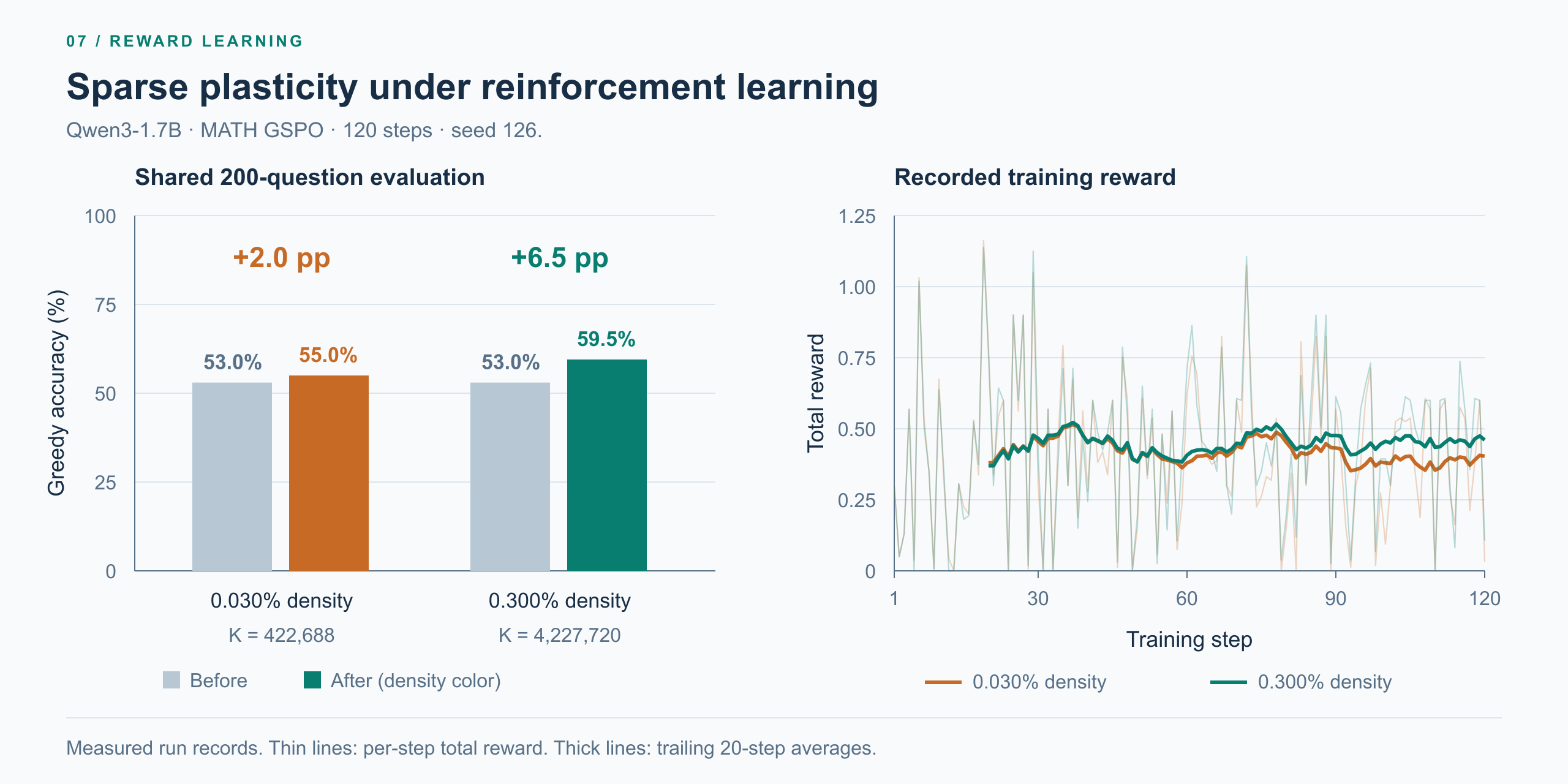
Figure 7. MATH GSPO records. Left: greedy accuracy on the shared 200-question evaluation slice. Right: recorded total reward at each training step, with a trailing 20-step mean. Each density uses seed 126.
Together, the SFT and RL results demonstrate a common learning interface. Supervised errors and reward signals both reach a small collection of independent connections, while the complete pretrained network carries out the computation.
The Engineering Conveniences of Coordinate Sparsity
The parameterization also determines what engineers must store, schedule, differentiate, and move. LoRA’s trainable-parameter percentage compresses four different bills into one attractive number: arithmetic, memory traffic, batching, and persistent state. Coordinate sparsity changes the objects behind each bill: learned projection pairs become indexed connection values, and the support becomes reusable execution metadata.
Where the Memory Savings Actually Happen
The pretrained network supplies the computation. Only the plastic connections carry trainable values, parameter gradients, and optimizer history.
Let \(N\) be the number of base-weight values and \(K\) the number of selected coordinates. The storage representation follows the parameterization directly:
The frozen base is stored once. The increment, its gradient, and its optimizer state are separate, coordinate-sized tensors. This places the savings at specific points in the training lifecycle.
Weights: reuse the base, allocate precision to the increments
The base retains its low-precision computation weights. A trainable vector holds the selected increments, and an FP32 master vector accumulates their updates before conversion to the computation dtype. Mixed-precision training uses master weights to preserve small updates across optimization steps; SparseLeaf allocates that precision to the connections that can change. The master copy therefore shrinks from \(N\) values to \(K\) values. Mixed Precision Training
Multiple tasks can reuse the same immutable base and maintain independent increment vectors. Saving an adapter records its support and values, while the base remains a separately stored asset. Once a receiver has the same base and support, a new adapter version can be transmitted as a replacement value vector. The savings appear in trainable weight storage, task-specific checkpoints, and version payloads.
Weight gradients: write the selected results directly
For \(Y=XW^\top\) and \(D=\partial\mathcal L/\partial Y\), full-parameter training forms \(G_W=D^\top X\), with one gradient value per weight. SparseLeaf’s backward operator instead writes
Each selected connection contributes one dot product across token positions. The operator writes those results directly into a length-\(K\) gradient buffer. The frozen base has no parameter-gradient buffer; the increment vector receives the accumulated gradient. This matches autograd’s distinction between differentiating through an operation and accumulating a gradient for one of its inputs. PyTorch Autograd: setting requires_grad
The saving begins at gradient generation: selected dot products replace the full weight-gradient multiplication, and \(K\) output writes replace \(N\). Microbatch accumulation then operates on the same \(K\) entries. Data-parallel replicas with an aligned fixed support synchronize those entries in a common coordinate order. The layer’s full input-gradient path continues to carry errors to earlier layers; the backward section below separates that computation from parameter-gradient generation.
Optimizer state: keep history only where learning can happen
Adam maintains a first moment and a second moment for each trainable value. With a sparse leaf, both histories have length \(K\). The optimizer creates the master vector and moment vectors in the leaf’s shape, updates them from its gradient, and writes back the new increment values. State allocation, per-step reads and writes, and optimizer checkpoints all follow the selected coordinates.
Using BF16 computation values and parameter gradients, an FP32 master copy, and two FP32 Adam moments gives the following logical tensor accounting. ZeRO uses this same separation of weights, gradients, master weights, and moments to explain the memory cost of mixed-precision Adam. ZeRO, §3.1
| Tensor | Full-parameter training | SparseLeaf |
|---|---|---|
| Complete computation weights / frozen base | \(2N\) bytes | \(2N\) bytes |
| Separate BF16 increments | — | \(2K\) bytes |
| Parameter gradients | \(2N\) bytes | \(2K\) bytes |
| FP32 master weights | \(4N\) bytes | \(4K\) bytes |
| Adam first moment | \(4N\) bytes | \(4K\) bytes |
| Adam second moment | \(4N\) bytes | \(4K\) bytes |
| Core tensor total | \(16N\) bytes | \(2N+16K\) bytes |
The full memory ledger adds coordinate metadata, activation storage, and operator workspace. An FP32 microbatch-accumulation buffer contributes another \(4K\) bytes while resident. In the core total above, the BF16 parameter-gradient buffer contributes \(2K\) bytes; accumulation and optimizer staging have their own lifetimes.
Return to the opening \(4096\times4096\) matrix with \(K=4096\) selected connections. Full-parameter training uses 256 MiB for the core tensors in the table. SparseLeaf uses 32 MiB for the base plus 64 KiB for the increment training state: 8 KiB of increments, 8 KiB of gradients, 16 KiB of master weights, and 32 KiB for the two moments. Flat INT32 coordinates add 16 KiB; CSR/CSC execution metadata is a separate allocation.
For standard LoRA with \(P=\sum_\ell r_\ell(m_\ell+n_\ell)\) factor values, the same accounting gives
Coordinate metadata adds \(B_S\) to SparseLeaf’s storage. Both representations reuse a frozen base. SparseLeaf makes the learning-state budget divisible into individual connections: removing one coordinate removes its increment, gradient, master value, and both moment entries. Every retained coordinate keeps an independent update direction. The memory budget follows the number of plastic connections while their combined update remains free to have high rank.
From skinny GEMMs to indexed accumulation
For \(T\) token rows, an unmerged LoRA layer computes
The adapter adds two dependent, skinny matrix multiplications. Reducing \(r\) narrows the first projection’s output dimension and the second projection’s reduction dimension. It shrinks their arithmetic and the work available to amortize scheduling and memory access. Each adapted gate, up, and down projection in an MoE expert carries this pair: six logical adapter multiplications per expert forward pass.
NVIDIA reports exactly this shape problem: even its heterogeneous batched GEMM underutilized the GPU on the first LoRA projection. Its implementation used split-K parallelism and an additional reduction kernel to improve utilization. A small factor matrix still required extra scheduling and reduction work. NVIDIA NIM implementation notes
The traffic arithmetic is revealing. For \(q\) token rows, factors of shapes \(r\times n\) and \(m\times r\), and \(b\) bytes per value, count one read of each factor and input, and one output write:
At one token and BF16, this model gives \(I_{\mathrm{traffic}}=r/(r+1)<1\). Intermediate tensors and output accumulation add traffic. The GPU executes shapes and memory transfers, not parameter-efficiency percentages.
SparseLeaf replaces the two learned contractions with a direct connection-wise operation:
A row-grouped kernel gathers the selected inputs, multiplies by their increment values, and accumulates directly into the corresponding outputs. The adapter has no rank-\(r\) intermediate \(Z\) to produce and consume. Its work is parallelized over tokens and coordinate blocks, instead of organized around two skinny learned projections.
Writing \(P=r(m+n)\), the forward arithmetic becomes \(2TK\) connection FLOPs in place of \(2TP\) factor FLOPs. Reducing \(K\) removes connections from the work list. It does not squeeze a learned projection into an increasingly narrow matrix shape. This targets both the amount of adapter work and its two-stage dependency.
From tenant–expert fragments to a shared coordinate schedule
With \(E\) routed experts, top-\(k\) routing, \(U\) tenants, and \(T\) token rows, balanced routing gives average group sizes
The base expert can process tokens from different tenants together. Independent tenant adapters have different factors, so their reuse groups are tenant–expert pairs.
Take \(T=512\), \(k=2\), \(E=64\), and \(U=16\). The base has 16 routed tokens per expert on average. The adapters have one routed token per tenant–expert cell on average. The apparent 512-token batch has become a grid of tiny adapter problems.
Grouped and fused kernels pack these fragments into fewer launches. They do not make different tenants reuse the same factor values. Increasing the expert count expands the collection of adapter states while reducing the token reuse available to each expert. Increasing the tenant count repeats that pressure.
Coordinate sparsity separates the execution structure from the tenant’s learned values. For a shared support \(S_e=\{(i_{e,k},j_{e,k})\}_{k=1}^{K_e}\) in one expert projection,
The indices and output-reduction pattern are identical across tenants. The tenant identifier selects a value vector, not a new pair of learned matrix contractions. This gives a fused kernel a scheduling key of expert plus coordinate block: traverse the expert’s token batch using one coordinate schedule and fetch each token’s tenant-specific values. In the example above, that schedule spans the expert’s 16 tokens instead of creating a separate projection chain for every one-token tenant–expert cell.
The same locality determines device placement. Put each increment on the device that owns its base-weight coordinate. Expert-local corrections join the existing expert output; tensor-parallel partial corrections join the base layer’s existing output reduction. There is no additional rank-dimensional intermediate to assemble across shards.
From adapter cache pressure to sparse value tables
Merging an adapter materializes a tenant-specific dense weight \(W_0+B_uA_u\). Different tenants then need different merged weights. Keeping one shared base instead leaves tenant-specific adapter computation on the serving path.
This is why multi-LoRA serving requires its own systems machinery. Punica introduces segmented gather matrix-vector multiplication to batch adapter work and group requests using the same factors. S-LoRA manages adapter weights and KV caches in one paged memory pool, adds heterogeneous kernels, and prefetches adapters. Adapter residency consumes memory that could otherwise hold longer contexts or more concurrent requests. Clustering requests by adapter improves reuse by changing who gets served together—and when. Punica, §§3–4, S-LoRA, §§4–5
The cost is a chain: more adapter identities mean more distinct weights, weaker per-adapter reuse, and more pressure on cache capacity and scheduling. Loading, eviction, transfer, and batching become part of the customization bill.
With a fixed shared coordinate support, tenant-specific storage is a value table. For one projection, let \(B_S\) be the shared coordinate-metadata size and \(b_w\) the number of bytes per learned value. Adapter storage for \(U\) resident tenants is
Each new tenant adds \(K\) values; the index table and reduction layout are reused. Smaller coordinate budgets therefore translate directly into smaller resident payloads, more room for KV caches, and fewer bytes on cache misses. Version updates use that same coordinate map, transmitting replacement increment values without rebuilding a factorized weight change.
For a materialized model version, patching touches the selected coordinates. A low-rank merge computes \(BA\) and writes a generally dense change; a coordinate patch writes \(K\) locations. SHiRA demonstrates this sparse-write approach through indexed adapter switching. Sparse High Rank Adapters, §3.2
From factor gradients to direct connection gradients
Let \(D=\partial\mathcal L/\partial Y\) and reuse \(Z=XA^\top\). LoRA’s backward pass contains
Freezing \(W_0\) removes its parameter gradient. It does not remove the dense multiplication \(DW_0\) that propagates learning signals to earlier layers. The adapter additionally contributes four skinny backward multiplications. CE-LoRA identifies this dense activation-gradient multiplication as the central computational bottleneck. CE-LoRA, §2.2
Count the forward and backward matrix multiplications of an interior linear layer, with both factors trained, unit adapter scaling, and two FLOPs per multiply-add:
Thus
An adapter with 0.1% of the layer’s parameters still uses approximately 66.77% of its full-training matrix-multiplication FLOPs. That is the arithmetic before accounting for the execution efficiency of the added skinny operations.
The activation bill is equally explicit: \(\nabla_A\mathcal L=C^\top X\) needs the full-width input \(X\). Making \(r\) smaller does not shrink \(X\); it must be retained or recomputed. LoRA-FA freezes the input projection precisely to remove this storage requirement. LoRA-FA, §§2.2–3.1
Parameter gradients, activation gradients, and saved activations are separate objects. Counting only the first obscures the training bottleneck.
SparseLeaf builds the parameter-gradient vector directly from the selected connections:
The kernel reduces along the token dimension and writes one result per coordinate. It produces neither a full weight-gradient matrix nor the factor-gradient chain through \(DB\). Gradient accumulation, Adam updates, and parameter-gradient synchronization operate on these \(K\) values.
The full activation gradient is
This preserves complete error transport through the pretrained network and makes the adapter correction a direct sparse accumulation. Under the same linear-layer arithmetic accounting,
The shared base computation is explicit; the adapter’s forward, parameter-gradient, and input-gradient work scales with the selected connections. The \(6TP\) factor-side work has become \(6TK\) connection-side work.
Activation retention also becomes an explicit support-layout problem. Define \(J(S)=\{j_k:k=1,\ldots,K\}\). A support-aware backward pass saves \(X_{:,J(S)}\) for the selected parameter dot products, requiring \(bT|J(S)|\) input-activation bytes. The engineer can optimize column coverage and reuse directly. Rank reduction offers no equivalent control over the full-width \(X\) needed to train \(A\).
From the rank-one floor to one-connection budgets
Rank is an integer. For a fixed collection \(\mathcal T\) of independently adapted matrices, the smallest nonzero standard LoRA allocation to every target is
The next smaller rank is zero: removing that matrix’s adapter. LoRA cannot spend three independent scalar parameters on a projection whose rank-one factorization costs thousands.
Consider Kimi K2’s routed experts. Its architecture has 61 layers, one dense layer, 384 routed experts per MoE layer, model width 7,168, and expert width 2,048. That gives 60 MoE layers. Kimi K2 technical report, §2.3
Allocate independent rank-\(r\) LoRA factors to the gate, up, and down projections of every routed expert. The resulting factor count is
The model activates eight routed experts per token, but the complete adapter contains factors for all 384. Token-level conditional computation does not shrink the all-expert checkpoint or its eventual optimizer state.
This is the rank-one trap: 637 million trainable values, yet each adapted projection is still restricted to one rank-one change. The granularity is simultaneously too expensive for tiny budgets and too restrictive for independent connection updates.
Coordinate sparsity breaks this floor while retaining the same projection coverage. Give every one of those 69,120 expert projections 16 selected entries in distinct rows and columns:
That is 576 times fewer trainable values than rank-one LoRA, and each projection’s update can attain rank 16. The budget is spent on independent connection changes across the same target matrices.
| Allocation per routed-expert projection | Trainable values | BF16 learned values | Two FP32 Adam moments |
|---|---|---|---|
| LoRA rank 1 | 637,009,920 | 1.274 GB | 5.096 GB |
| LoRA rank 8 | 5,096,079,360 | 10.192 GB | 40.769 GB |
| SparseLeaf: 16 coordinates | 1,105,920 | 2.212 MB | 8.847 MB |
Derived allocation and storage accounting for the same 69,120 projections. Decimal units; learned values use two bytes each and the moment pair uses eight. Shared coordinate metadata is stored separately.
With BF16 values and gradients, an FP32 master copy, and two FP32 Adam moments, the training-state totals are \(16P_1=10.192\) GB for rank-one LoRA and \(16K=17.695\) MB for this coordinate allocation. For 100 resident tenants, their BF16 value payloads are 127.402 GB and 221.184 MB, respectively.
One extra LoRA rank purchases \(m+n\) factor values in a target matrix. One extra SparseLeaf coordinate purchases one connection. That granularity lets an engineer allocate a global budget across layers and experts without treating a rank-one adapter as an indivisible minimum purchase.
The engineering correspondence is direct: indexed accumulation replaces skinny projection chains; shared supports provide reusable multi-tenant schedules; selected dot products produce the learning gradients; and coordinate budgets control resident state and update payloads. These conveniences follow from making the connections themselves plastic.
From Parameter Compression to Synaptic Plasticity
The 4,096-entry example at the beginning captures the central idea: an update can be small in coordinates and large in rank.
The task construction turns that idea into a strict loss separation. The optimizer shows how the selected connections receive their native gradients. The allocation problem asks which connections are worth making plastic. The experiments show what those connections learn under supervision and reward.
Together, they suggest a different organizing principle for parameter-efficient learning: spend the budget on choosing plastic connections, and preserve their freedom to create independent changes.
SparseLeaf makes the support of learning an explicit part of the optimization problem. It preserves the pretrained network’s computation, gives selected connections independent increments, and lets those increments form high-rank updates.
The important unit is the plastic connection. Its location determines where a change enters the network. Its gradient determines what the task asks it to do. Its optimizer state records how that request develops over time. Many such local changes can combine into a high-rank transformation.
Dense capacity. Sparse plasticity. High-rank updates.
Appendix A. The First-Step Geometry of Gaussian LoRA Initialization
Take a deterministic forward pass without adapter dropout, unit adapter scaling, ordinary gradient descent, \(B_0=0\), and independent entries \(A_{0,ij}\sim\mathcal N(0,1/r)\). The base-model gradient \(G\) is fixed and independent of \(A_0\).
Write
Then \(\mathbb E Q=I_n\). For one Gaussian vector,
because each diagonal entry has expectation
and off-diagonal expectations vanish. Independence gives
Consequently,
The effective first update is \(\Delta W_1=-\eta GQ\), so
Averaging \(M\) independent initialized updates divides this mean squared deviation by \(M\). The factorization thus has both an exact mean update and a computable distribution around it.
The initial-subspace projection
For \(1\le r\le n\), a Gaussian \(A_0\) has full row rank almost surely. Its row-space projector \(\Pi_0\) satisfies \(\Pi_0^\top=\Pi_0\), \(\Pi_0^2=\Pi_0\), and \(\operatorname{tr}\Pi_0=r\). Rotational invariance implies \(\mathbb E\Pi_0=cI_n\); taking traces gives \(c=r/n\).
Orthogonal projection onto \(\mathcal T_0=\{HA_0\}\) acts on each row of \(G\), so
Idempotence then yields
This isolates the missing-direction cost from the random scaling of the unnormalized Gram matrix.
Appendix B. A Sparse Mask Can Produce a High-Rank Step
For one example in a linear layer, the weight gradient is an outer product:
With a binary coordinate mask \(M\), a selected-coordinate gradient-descent step is
Take nonzero entries in \(\delta\) and \(x\), and nonzero \(\eta\). The two diagonal matrices are invertible, giving
For a square layer with \(M=I_d\), the step changes \(d\) coordinates and has rank \(d\). The coordinate mask has converted a rank-one gradient into a sparse full-rank update. Sparsity and rank describe different structures even at the level of an individual learning step.
References
- Hu, E. J., et al. (2021). LoRA: Low-Rank Adaptation of Large Language Models. arXiv:2106.09685; ICLR 2022.
- Eckart, C., and Young, G. (1936). The Approximation of One Matrix by Another of Lower Rank. Psychometrika, 1, 211–218.
- Zeng, Y., and Lee, K. (2024). The Expressive Power of Low-Rank Adaptation. ICLR.
- Aghajanyan, A., Gupta, S., and Zettlemoyer, L. (2021). Intrinsic Dimensionality Explains the Effectiveness of Language Model Fine-Tuning. ACL-IJCNLP.
- Matsuzaki, M., Honkura, N., Ellis-Davies, G. C. R., and Kasai, H. (2004). Structural basis of long-term potentiation in single dendritic spines. Nature, 429, 761–766.
- Guo, D., Rush, A. M., and Kim, Y. (2021). Parameter-Efficient Transfer Learning with Diff Pruning. ACL-IJCNLP.
- Rios, J., Dognin, P., Luss, R., and Natesan Ramamurthy, K. (2025). Sparsity May Be All You Need: Sparse Random Parameter Adaptation. Findings of EMNLP.
- Bhardwaj, K., et al. (2024; revised 2025). Sparse High Rank Adapters. arXiv:2406.13175.
- Liu, X., et al. (2025). Refining Salience-Aware Sparse Fine-Tuning Strategies for Language Models. ACL.
- Kingma, D. P., and Ba, J. (2015). Adam: A Method for Stochastic Optimization. ICLR.
- Duchi, J., Hazan, E., and Singer, Y. (2011). Adaptive Subgradient Methods for Online Learning and Stochastic Optimization. Journal of Machine Learning Research, 12, 2121–2159.
- Hayou, S., Ghosh, N., and Yu, B. (2024). The Impact of Initialization on LoRA Finetuning Dynamics. NeurIPS.
- Shuttleworth, R., Andreas, J., Torralba, A., and Sharma, P. (2024; revised 2025). LoRA vs Full Fine-tuning: An Illusion of Equivalence. arXiv:2410.21228, version 3.
- Williams, R. J. (1992). Simple statistical gradient-following algorithms for connectionist reinforcement learning. Machine Learning, 8, 229–256.
- Mukherjee, S., Yuan, L., Hakkani-Tür, D., and Peng, H. (2025). Reinforcement Learning Finetunes Small Subnetworks in Large Language Models. arXiv:2505.11711, version 2.
- Jacot, A., Gabriel, F., and Hongler, C. (2018). Neural Tangent Kernel: Convergence and Generalization in Neural Networks. NeurIPS.
- Nutini, J., Schmidt, M., Laradji, I., Friedlander, M., and Koepke, H. (2015). Coordinate Descent Converges Faster with the Gauss-Southwell Rule Than Random Selection. ICML.
- Sung, Y.-L., Nair, V., and Raffel, C. (2021). Training Neural Networks with Fixed Sparse Masks. NeurIPS.
- Verma, S., et al. (2024). Seamlessly Deploying a Swarm of LoRA Adapters with NVIDIA NIM. NVIDIA Technical Blog, June 7.
- Chen, L., Ye, Z., Wu, Y., Zhuo, D., Ceze, L., and Krishnamurthy, A. (2023). Punica: Multi-Tenant LoRA Serving. arXiv:2310.18547; MLSys 2024.
- Sheng, Y., et al. (2023; revised 2024). S-LoRA: Serving Thousands of Concurrent LoRA Adapters. arXiv:2311.03285; MLSys 2024.
- Chen, G., He, Y., Hu, Y., Yuan, K., and Yuan, B. (2025). CE-LoRA: Computation-Efficient LoRA Fine-Tuning for Language Models. arXiv:2502.01378.
- Zhang, L., Zhang, L., Shi, S., Chu, X., and Li, B. (2023). LoRA-FA: Memory-efficient Low-rank Adaptation for Large Language Models Fine-tuning. arXiv:2308.03303, version 1.
- Kimi Team (2025; revised 2026). Kimi K2: Open Agentic Intelligence. arXiv:2507.20534.
- Hayou, S., Ghosh, N., and Yu, B. (2024). LoRA+: Efficient Low Rank Adaptation of Large Models. ICML, PMLR 235, 17783–17806.
- Wang, S., Yu, L., and Li, J. (2024). LoRA-GA: Low-Rank Adaptation with Gradient Approximation. arXiv:2407.05000; NeurIPS.
- Meng, F., Wang, Z., and Zhang, M. (2024; revised 2025). PiSSA: Principal Singular Values and Singular Vectors Adaptation of Large Language Models. arXiv:2404.02948; NeurIPS 2024.
- Hao, Y., Cao, Y., and Mou, L. (2024). Flora: Low-Rank Adapters Are Secretly Gradient Compressors. ICML, PMLR 235, 17554–17571.
- Kalajdzievski, D. (2023). A Rank Stabilization Scaling Factor for Fine-Tuning with LoRA. arXiv:2312.03732.
- Yen, J.-N., et al. (2025). LoRA Done RITE: Robust Invariant Transformation Equilibration for LoRA Optimization. ICLR; arXiv:2410.20625.
- Paischer, F., Hauzenberger, L., Schmied, T., Alkin, B., Deisenroth, M. P., and Hochreiter, S. (2025). Parameter Efficient Fine-tuning via Explained Variance Adaptation. NeurIPS; arXiv:2410.07170.
- Wang, Z., Liang, J., He, R., Wang, Z., and Tan, T. (2025). LoRA-Pro: Are Low-Rank Adapters Properly Optimized?. ICLR; arXiv:2407.18242.
- Micikevicius, P., et al. (2018). Mixed Precision Training. ICLR.
- PyTorch Contributors (2026). PyTorch Autograd: setting requires_grad. PyTorch 2.14 documentation.
- Rajbhandari, S., Rasley, J., Ruwase, O., and He, Y. (2020). ZeRO: Memory Optimizations Toward Training Trillion Parameter Models. arXiv:1910.02054, version 3.